MATLAB package for stress inversion from focal mechanisms

Version 1.0.10, Last update: 22.04.2015

Authors:

Patricia Martínez-Garzón <patricia@gfz-potsdam.de>
Grzegorz Kwiatek <kwiatek@gfz-potsdam.de>

Original SATSI library code by Jeanne Hardebeck and Andy Michael (website); see Hardebeck and Michael [2006] for details. MSATSI package uses MATLAB routine sh.m for appropriate calculation of the horizontal stresses, developed by Bjorn Lund and John Townend (website); see also Lund and Townend [2007] for details. The extensive description of the package together with examples is presented in Martínez-Garzón et al. [2014]. If you find the MSATSI useful in your research you can acknowledge our work by providing a reference to the following works:

Martínez-Garzón, P., Kwiatek, G., Ickrath, M. and M. Bohnhoff (2014). MSATSI: A MATLAB package for stress inversion combining solid classic methodology, a new simplified user-handling and a visualization tool. Seismol. Res. Lett., 85,4, doi: 10.1785/0220130189. Go to: Full article (web view); Download: Full article (pdf) through GeoScienceWorld.

Hardebeck, J. L., and Michael, A. J. (2006). Damped regional-scale stress inversions: Methodology and examples for southern California and the Coalinga aftershock sequence, J. Geophys. Res. Solid Earth 111, no. B11, B11310, doi 10.1029/2005JB004144.

Lund B. and Townend, J., (2007). Calculating horizontal stress orientations with full or partial knowledge of the tectonic stress tensor, Geophys. J. Int., 170, 1328-1335, doi: 10.1111/j.1365-246X.2007.03468.x.

Also, you can let us know on your publications using MSATSI packake. We are happy to advertise them at this website!

Download

The newest version of MSATSI package can requested by filling the following form. After submitting the form, the email message with download link will be sent to you. In case you don’t receive the letter after a couple of minutes, please firstly check your spam folder and then contact us!

Changelog

The current version of MSATSI package is 1.0.10:

1.0.10 (Release data: 22.04.2015) Correction to path handling in Windows systems
1.0.9 (Release data: 27.03.2015) Various corrections to account for path/file handling in Mac/Linux versions.
1.0.8 (Release date: 04.02.2015) SilentMode and SaveImage options added. Small corrections to existing code. Correction to the best solution of satsi2d.
1.0.7 (Release date: 02.06.2014) Correction to stereonet grid plotting routine in msatsi_plot.m
1.0.6 (Release date: 01.06.2014) PDF/Word documentation added, binaries updated.
1.0.5 (Release data: 22.10.2013) Correction to the small bug introduced in 1.0.4
1.0.4 (Release date: 19.09.2013) Correction to the msatsi.m parameter FractionValidFaultPlanes.

1.0.3 (Release date: 24.08.2013) Initial release.

Table of contents

1. Introduction
2. Installation
   1. Installation for Microsoft Windows
   2. Installation for Linux / Mac
   3. Important notice to all MSATSI users
3. Quick start guide
   1. Performing stress inversion
   2. Displaying stress inversion results
4. Package documentation
   1. Content of the package
   2. Input data for msatsi routine
   3. Running the stress inversion with msatsi routine
   4. Properties of msatsi routine
   5. Stress inversion output
   6. Input data for msatsi_plot routine
   7. Running msatsi_plot
   8. msatsi_plot properties
5. Examples
6. Compilation of SATSI for different platforms
   1. Compilation for Linux platform
   2. Compilation for Windows platform
   3. Compilation for Mac platform
7. References

1. Introduction

MSATSI is a MATLAB software package that allows performing the stress inversion using earthquake focal mechanisms. MSATSI is based on the C library SATSI created by Hardebeck and Michael (2006) (http://earthquake.usgs.gov/research/software/#SATSI). MSATSI provides a framework for calculating the deviatioric stress tensor together with its uncertainties using bootstrap resampling method. It also allows displaying the stress inversion results using a variety of plots.

The MSATSI package is composed of two MATLAB functions. The first one msatsi.m performs actual stress inversion and the second one, msatsi_plot.m, provides the graphical visualization of stress inversion results calculated with MSATSI.

Main features of MSATSI package are:

• Simple and comprehensive handling of input and output stress inversion data.
• Variety of graphical representations of the stress inversion results: stereonets, stereotraces, profiles, world stress map-alike plots, stereomaps and stereovolumes.
• Versatile and adjustable graphical output
• User friendly interface through the intensive use of MATLAB properties.

The details of the software package are described in Martínez-Garzón et al. [2014].

2. Installation

In the first step, please use the form above to download the current version of the package.

2.1 Installation for Microsoft Windows

1. Unpack downloaded version of MSATSI to some directory.
2. Add the root folder of the package (i.e. the location containing msatsi.m and msatsi_plot.m functions) to the MATLAB search path (File>Set Path option in MATLAB main menu). Alternatively, copy both m-files together with seven executable files (*.exe) to the directory already included in your MATLAB search path.
3. Done!

2.2 Installation for Linux / Mac users

1. Unpack downloaded version of MSATSI to some directory.
2. Add the root folder of the package (i.e. the location containing msatsi.m and msatsi_plot.m functions) to the MATLAB search path (File>Set Path in MATLAB main menu).
3. Depending on your platform, proceed to the appropriate subfolder of ./bin directory and copy seven executable files into the place where you placed msatsi.m and msatsi_plot.m routines. You can delete the existing *.exe files, as these are executables for Microsoft Windows platform that are of no use for Linux / Mac users. Alternatively, copy both m-files together with executable files appropriate for your platform to the directory already included in your MATLAB search path.
4. Done!

2.3 Important notice to all MSATSI users

Executable files appropriate for each platform (Microsoft Windows, Linux or Mac) must be located in the same directory where msatsi.m and msatsi_plot.m files are stored, otherwise msatsi function will not work properly.

3. Quick start guide

This quick start guide provides the basics of MSATSI package usage. For a detailed description of stress inversion using msatsi.m routine and parameters controlling the inversion procedure, the user is referred to sections 4.2-4.5. For the description of msatsi_plot.m funtion and parameters controlling the graphical output, the MSATSI user is referred to Sections 4.6-4.8 of this documentation.

Obtaining the stress orientation from focal mechanisms using MSATSI basically consists of the three steps. In the first step we prepare (or as in the case of this quick start tutorial – simply load) the input data table containing information about focal mechanisms. In the second step we perform the actual stress tensor inversion using msatsi.m function. Finally, after successful completion of the stress inversion, we will display the obtained results using msatsi_plot.m function.

3.1 Performing stress inversion

When in MATLAB, change the current directory to ./examples/example1D. This folder contains example input focal mechanism data from the North Anatolian Fault Zone (dip direction, dip angle and rakes of numerous earthquakes that occurred along the fault zone. The input data table in a form of MATLAB matrix is stored in the INPUT_example1D.mat. This file contains focal mechanism data divided arbitrarily into 27 temporal divisions (in the formal documentation of MSATSI package presented in this documentation the term ‘division’ is referred as ‘grid point’) containing 70 seismic focal mechanisms. This division was made in order to display with the stress inversion the changes in the stress field orientation along the major fault plane.

Once we are in the ./examples/example1D directory, type in MATLAB command prompt:

load('INPUT_example1D.mat')

This call will load the input data table containing focal mechanism data. New variable example1d should be now visible in MATLAB workspace. Alternatively, you can also load the text version of the table by calling:

example1d = load('INPUT_example1D.txt)

The loaded file is a matrix containing dip directions, dip angle and rakes of faults (columns 3-5 of the matrix). The first two columns contain the information on the segment number (grid point) the particular focal mechanism belongs to (in fact, the first column contains only zeros with the second column changing from 0 to 26). As you noticed, there is no direct information on location of specific seismic events, but only the information about the segment (grid point) the particular focal mechanism is attributed to. Fault plane solutions from each segment (grid point) will be inverted for the stress tensor, therefore we expect obtain a set of 27 stress tensors reflecting the direction of cardinal stress axes along the North Anatolian fault plane.

Now let’s finally call the stress inversion by typing:

OUT = msatsi('example1',example1D,'BootstrapResamplings',2000)

This will perform a complete stress inversion together with bootstrap uncertainty assessment. The first input parameter is the project name. For each project, a separate project directory is created during inversion. This folder contains input and output data as well as additional intermediate graphical output if requested by the user. The second parameter is simply the input table we loaded with the load function. The last ParameterName-ParameterValue pair ‘BootstrapResamplings’ modifies the default number of bootstrap resampling by requesting to perform 2000 bootstrap resamplings of the original input data instead of (default) 500.

The inversion procedure with MSATSI will take some time. The details of the inversion procedure are described in details in Martínez-Garzón et al. [2014]. In the first stage, the tradeoff parameter is calculated using an automated procedure. In the second step, the actual stress inversion is performed and the best stress tensors are found for each grid point. Finally, the input dataset is resampled using bootstrap procedure and the confidence intervals of stress tensor axes are found. The results of stress inversion and uncertainty assessment are stored in a project directory (in our case inside example1 folder) in MAT file called example1_OUT.mat (as you noticed, the name of MAT file depends on project name). However, the content of output MAT file is also returned directly by msatsi.m function as a structure array. We therefore grab the stress inversion result in OUT structure.

There are a number of input inversion parameters possible to modify by providing additional property name-propery value pairs. For a comprehensive overview of all parameters we refer to Section 4.4 of this documentation.

As example, consider the case when one wants to calculate the 68% confidence intervals, but by default msatsi calculates 95% confidence intervals. This can be easily modified by specifying additional parameter ‘ConfidenceLevel’:

OUT = msatsi('example1',example1D,'BootstrapResamplings',2000,'ConfidenceLevel',68)

3.2 Displaying stress inversion results

The stress inversion results may be graphically represented in a variety of ways using msatsi_plot routine. Here, we present changes in the stress field orientation as a profile plot. In order to create a picture, we now call msatsi_plot routine:

msatsi_plot('example1','profile','Title',{'Changes of S1-S3 along NAFZ'})

where the first parameter is either the directory containing the solution (e.g. ‘example1’) or directly the output structure array from the call to msatsi.m function, i.e. the following syntax should give the same results, provided that OUT structure array is an outcome of the relevant stress inversion presented in Section 3.1:

msatsi_plot(OUT,'profile','Title',{'Changes of S1-S3 along NAFZ'})

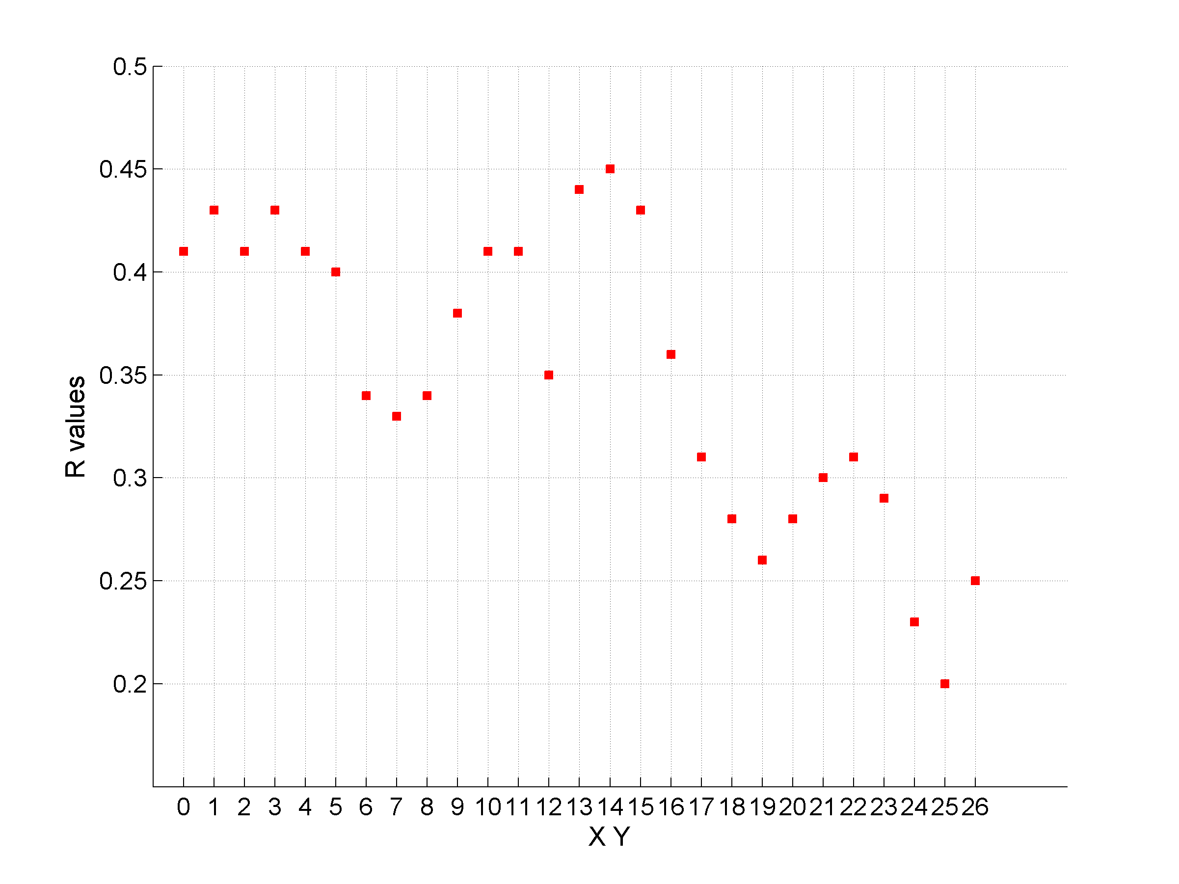
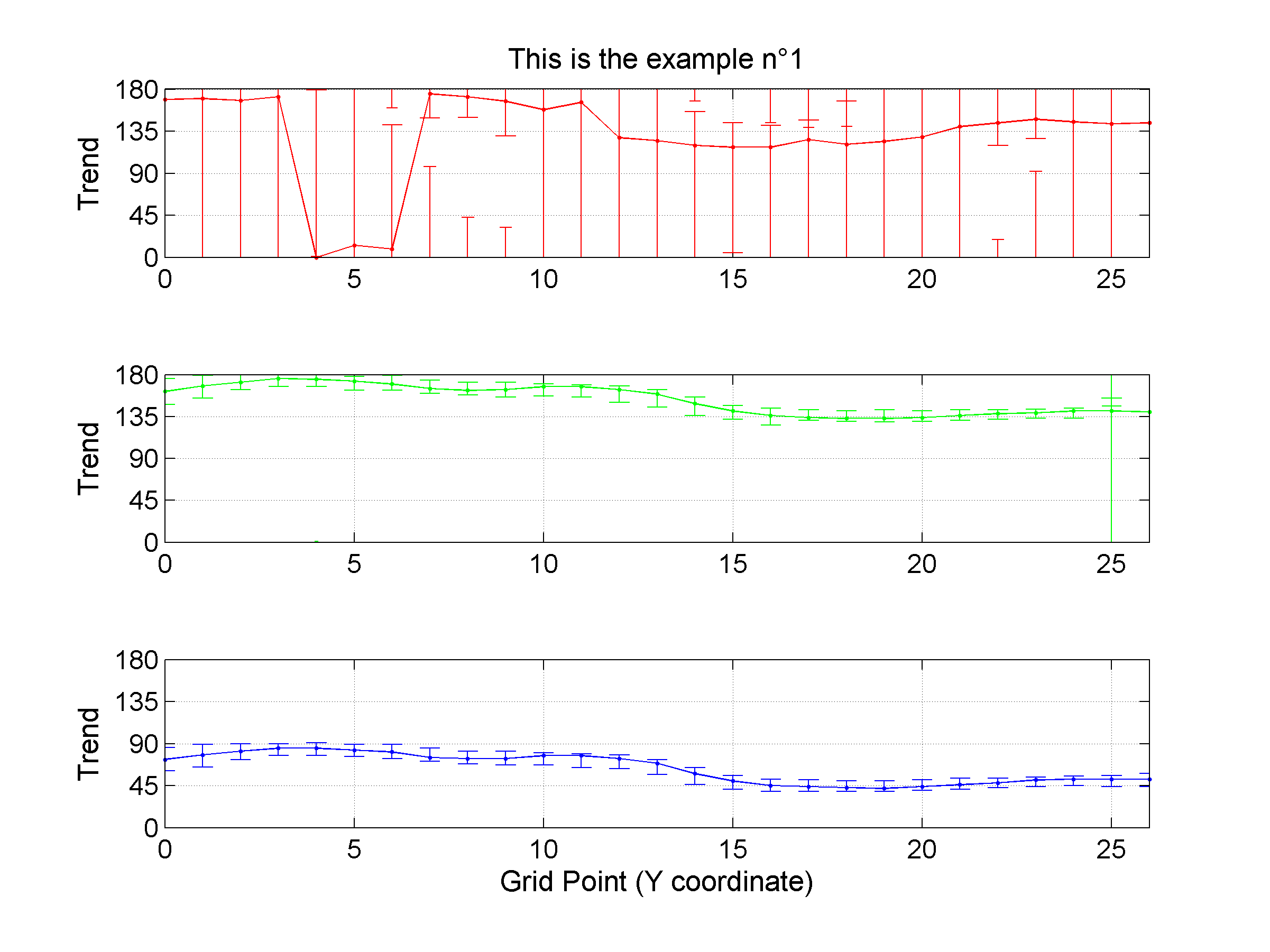
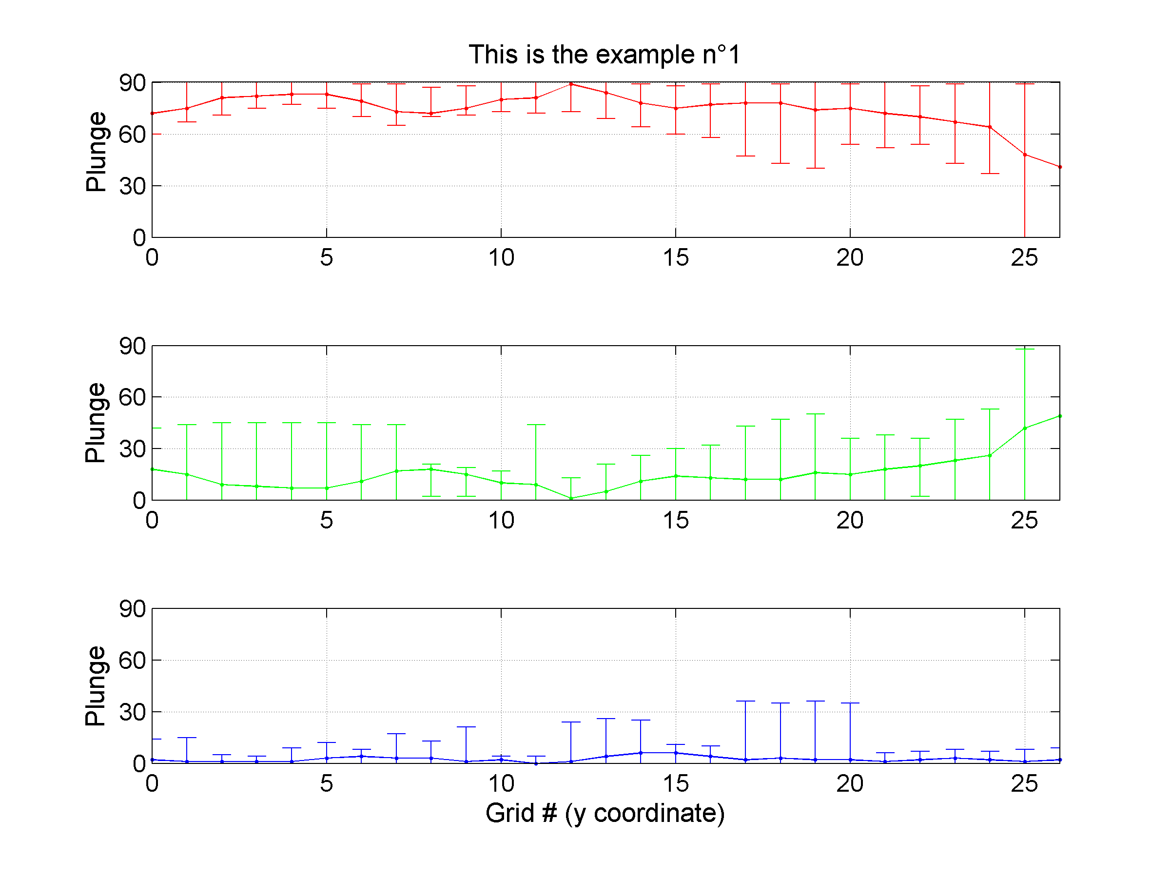
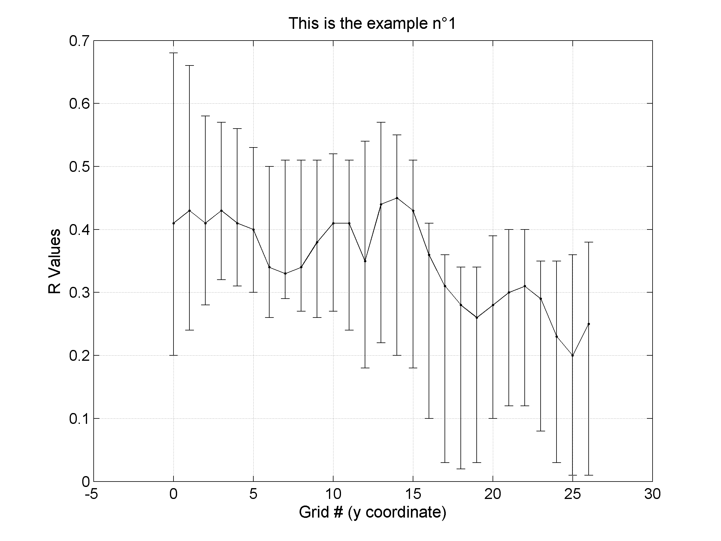
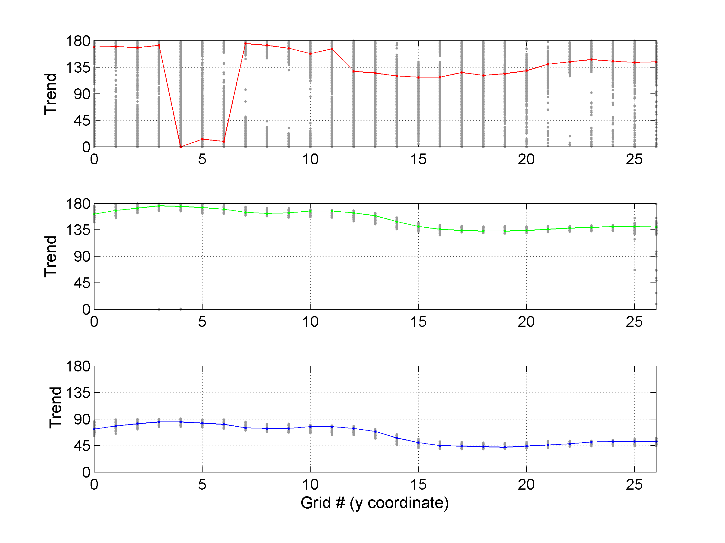
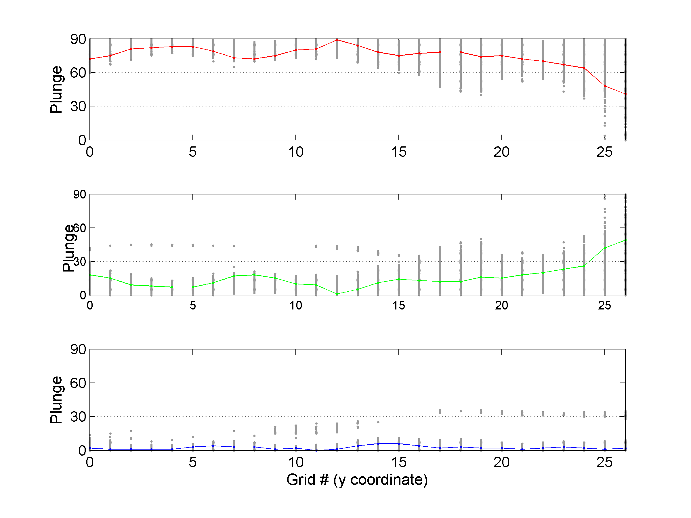
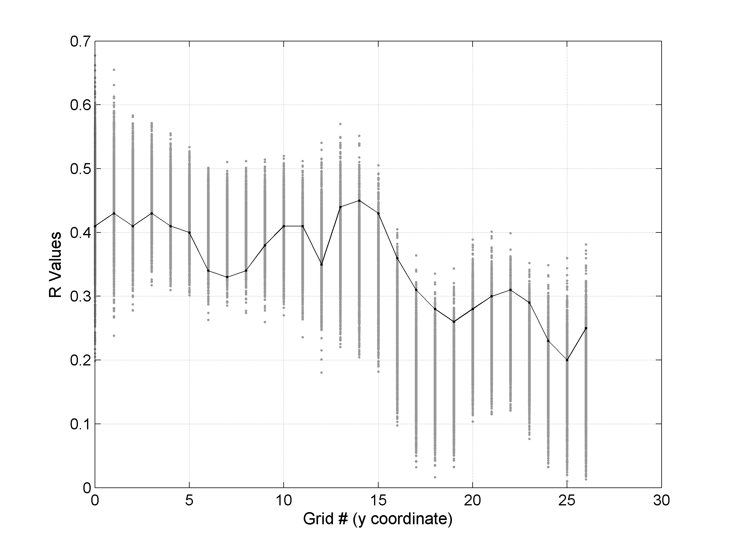
The second parameter specifies the plot type to create. The ‘profile‘ option creates three pictures: one for variations of the trend angles , second analogous picture for variations in plunge, and a third one with variations in R (stress ratio coefficient). Bootstrap-aided 95% confidence intervals are represented by default with error bars. With the property ‘Title’, we have written the title we wished on top of each figure.

Various, highly customizable plots can be created using msatsi_plot.m by specifying additional properties. We refer to Sections 4.6-4.8 of this document for details.

The additional examples are presented in Section 5 of this document. Good luck!

4. Package documentation

This part contains the information on input and output formats as well as the description of the two core routines forming MSATSI package: msatsi.m and msatsi_plot.m.

4.1 Content of the package

The unzipped MSATSI package contains the following files and folders:

Location	Description
./	The root directory contains msatsi.m and msatsi_plot.m routines together with auxiliary SATSI executable files compiled for Microsoft Windows platform. Files for other platforms are located in the ./bin subfolder and MUST be copied to the root directory before using msatsi.m script when platform different the Microsoft Windows is used. Both m-files and executables should be kept together for a proper functioning of the package.
./bin	This folder contains SATSI executables precompiled for Windows, Linux and Mac platforms. If MATLAB is running on other platform than Microsoft Windows, executable files in the root folder (./) should be replaced with appropriate executable files either from ./bin/linux or ./bin/mac for Linux and Mac, respectively. By default, the root directory (./) contains executables for Microsoft Windows platform (*.exe).
./examples	This directory provides illustrations of the usage of MSATSI package. Examples 1D-3D cover the cases presented in the paper of Martínez-Garzón et al. (2014). Example 0D presents additional stress inversion together with graphical output not presented in the manuscript. Short descriptions are available in each subfolder of the ./examples directory as well as input and output data.
./src	Contains modified C code from original SATSI package available at USGS website. Instructions on how to compile the package for different platforms is provided inside of the directory. For the user's convenience, the compiled programs for different platforms are available in ./bin directory.

4.2 Input data for msatsi routine

The input matrix for stress tensor inversion varies whether inversion using 0D/1D/2D grid or 3D/4D grid is performed. For 0D-2D case, the input matrix is of n-by-5 size where n is the number of input data (i.e. focal mechanisms). Each row of the input data matrix contains the following data:

[X Y DIP_DIR DIP_ANGLE RAKE]

where the columns are:

Column name	Column description
X,Y	Grid point indexes (unsigned integer values)
DIP_DIR	Dip direction (degrees)
DIP_ANGLE	Dip angle (degrees)
RAKE	Rake (degrees)

NOTE: Please note that the input parameters for the fault plane solution is dip direction, dip angle and rake and NOT the strike, dip angle and rake.

An example of input data file for 0D/1D/2D cases can be found in ./examples/example1D/INPUT_example1D.txt or the corresponding MAT file located in the same directory. The input stress inversion data for 3D/4D case is slightly different as it has two additional columns:

[X Y Z T DIP_DIR DIP_ANGLE RAKE]

where Z and T are two additional grid point indexes. For an example of input file for 3D/4D, see ./examples/example3D/INPUT_example3D.txt.

4.3 Running the stress inversion with msatsi routine

Be sure that you are placed in the directory containing msatsi.m and the appropriate executable files.

First, load or create your input file. For example, load the input data file from ./examples/example1D directory:

load('INPUT_example1D.mat')

Run the inversion editing the desirable initial parameters, for example:

OUT = msatsi('example1',example1D,'BootstrapResamplings',2000)

Now you have to wait a bit for inversion to finish.

4.4 Properties of msatsi routine

The initial parameters of the inversion with the msatsi.m routine can be modified using various PropertyName-PropertyValue pairs.

The available properties of msatsi.m routine are gathered in a table below:

Property Name	Constraints	Default Value	Description
BootstrapResamplings	Scalar > 0	500	It defines number of bootstrap resamplings to be performed
Caption	String	NULL	Additional comments to be included
ConfidenceLevel	0 < Scalar < 100	95	Percentage of confidence interval of the results
Damping	'on' | 'off'	'on'	It switches on/off the calculation of damping parameter and tradeoff curve
DampingCoeff	Scalar >= 0	0	Value of the damping coefficient used (defined as 0 before calculation is activated, set automatically to 0 if damping is 'off')
FractionValidFaultPlanes	0 <= Scalar <= 1	0.5	Fraction of valid fault planes from the input data. If fault plane is selected randomly from the two possible options (typical case for fault planes from seismic data), then = 0.5
MinEventsNode	Scalar > 0	20	Minimum of events per grid point to perform stress inversion
PTPlots	'on' | 'off'	'off'	Switches on/off the plotting of P and T axes for every grid point
TimeSpaceDampingRatio	Scalar > 0	1	Property used in 4D case: If there is no difference in treatment for columns Z and T of input data, then = 1

4.5 Stress inversion output

During call of msatsi routine, the folder is created in the current MATLAB directory containing input and output inversion files. This folder contains the following files:

Filename	Description
.sat	Contains the data from the input file.
_tradeoff.png	Only created if damping is activated for the stress inversion. The file contains tradeoff curve and selected damping parameter.
.out	Contains the output of satsi2d.exe/satsi4d.exe. The first part reflects best solution data for each grid point: [X Y See Sen Seu Snn Snu Suu] where See Sen Seu Snn Snu Suu are the 6 independent components of deviatoric stress tensor (in case of 3D/4D problem, two columns more are present: [X Y Z T See Sen Seu Snn Snu Suu]). The second part gives for each input focal mechanism the magnitude of shear traction vector and deviation between predicted and calculated slip.
.slboot_tensor	The file is an output of bootmech2d.exe/bootmech4d.exe. It contains the (deviatoric) stress tensor coordinates for each grid and each bootstrap performed. The columns are [X Y See Sen Seu Snn Snu Suu] for 0D/1D/2D problem, and [X Y Z T See Sen Seu Snn Snu Suu] for 3D/4D.
.slboot_trpl	This file is a second output of bootmech2d.exe/bootmech4d.exe. It contains trend and plunge of principal stress axes for each grid and each bootstrap performed. The columns are [X Y Phi Tr1 Pl1 Tr2 Pl2 Tr3 Pl3] for 0D/1D/2D and [X Y Z T Phi Tr1 Pl1 Tr2 Pl2 Tr3 Pl3] for 3D/4D.
.summary	Contains output from bootuncert.exe. It contains best, minimum and maximum values for PHI, and the principal stress axes for each grid point. The columns are: [PhiBest PhiMin PhiMax Tr1Best Tr1Min Tr1Max Pl1Best Pl1Min Pl1Max Tr2Best Tr2Min Tr2Max Pl2Best Pl2Min Pl2Max Tr3Best Tr3Min Tr3Max Pl3Best Pl3Min Pl3Max]
.summary_ext	It forms another output of bootuncert.exe. It contains for each grid point the bootstrap resamplings included within the specified confidence interval. Here, regardless of the dimensionality of the problem, the columns are: [X Y Z T PHI TR1 PL1 TR2 PL2 TR3 PL3].
_OUT.mat	This structure array contains input parameters for the stress inversion as well as the resulting output data together with bootstrap uncertainty assessment . The structure contains (sizes of matrices presented are only example, the actual size may change depending on performed inversion): Out.Damping: 1 (If damping is 'off', then = 0, if damping is 'on', then =1) Out.DampingCoeff: 2.8 Final damping coefficient used after calculation. Out.ConfidenceLevel: 95 Out.FractionValidFaultPlanes: 0.5000 Out.MinEventsNode: 20 Out.BootstrapResamplings: 2000 Out.Caption: '(example1)' Out.TimeSpaceDampingRatio: 1 Out.PTPlot: 0 Out.SLBOOT_TENSOR: [54000x8 double] Information and structure equal to 'example1.slboot_tensor' Out.SLBOOT_TRPL: [54000x9 double] Information and structure equal to 'example1.slboot_trpl' Out.BOOTST_EXT: [51289x11 double] Information and structure equal to 'example1.summary_ext' Out.INPUT_TABLE: [1890x5 double] Information and structure equal to 'example1.sat' Out.SUMMARY_TABLE: [27x21 double] Information and structure equal to 'example1.summary' Out.GRID: [[27x3 double] Contains the order of the grid-points in which the inversion results are sorted (for example, in .summary file). If SI is 0D/1D/2D, the columns are [X Y Nevents], where Nevents is the number of focal mechanisms included in each grid point. If SI is 3D/4D, the columns are: [X Y Z T Nevents].

4.6 Input data for msatsi_plot routine

By default, the msatsi_plot.m program is using the output data created by msatsi.m. Thus, no additional input file needs to be created for msatsi_plot.m routine.

4.7 Running msatsi_plot

There are two ways of calling the msatsi_plot.m. Firstly, one can specify the directory containing the stress inversion results. In this case, the folder must be located in the current MATLAB directory. The example call could look as follows:

msatsi_plot('example1', plottype, 'PropertyName', PropertyValue, ...)

where ‘example1’ is the directory located in the current MATLAB folder. The other way of producing the graphical output is to call the msatsi_plot.m routine with the output structure array derived by msatsi.m:

msatsi_plot(Out, plottype, 'PropertyName', PropertyValue, ...)

where Out is a structure array returned by the previous call to msatsi.m routine:

Out = msatsi(...)

The second obligatory parameter, plottype, is the type of the plot. There are five different plots available:

PlotType	Dimensions	Description
'stereonet'	0D-1D	Suitable to represent the 0D-1D stress inversion results (e.g. temporal changes, changes of stress field orientation along the fault plane etc.). The direction of the principal stress axes is plotted using stereonet and lower hemisphere projection. R values for each grid point are plotted in a separate figure
'profile'	1D	This plot is composed of three figures showing changes in plunge and trend of the principal stress axes and R for each grid point.
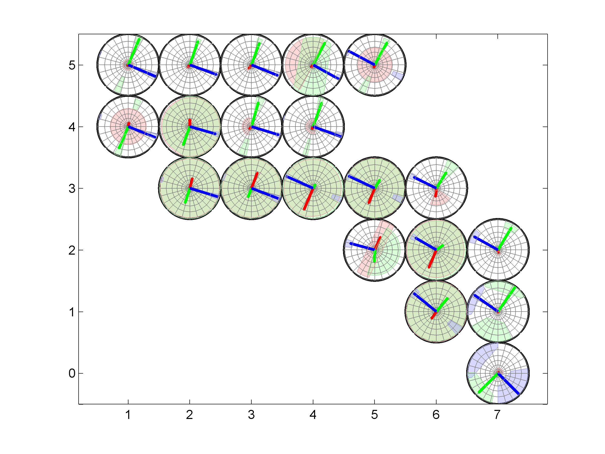
'stereomap'	2D	Appropriate for visualization of 2D stress inversion results (e.g. surface distribution). Directions of principal stress axes for each grid point forming a map are plotted using the stereonet. 2D distribution of R values is shown as a separate figure.
'wsm'	2D	This option creates a 2D plot compatible to those created by World Stress Map project (Heidbach et al., 2010). It shows the directions of the maximum horizontal stress according to the respective stress faulting regime classification criteria (Zoback, 1992)
'stereovolume'	3D	It is appropriate for 3D stress inversion data. The results are presented as 3D plot with cardinal stress axes directions pointing according to their trends and plunges. The idea is analogous to “stereomap” but extended to 3D

To modify the graphical characteristics of obtained plots, the user may specify additional PropertyName-PropertyValue pairs to adjust the graphical output.

4.8 msatsi_plot properties

The design of the plots created with msatsi_plot.m can be significantly modified using a number of PropertyName-PropertyValue pairs. The available msatsi_plot.m properties are gathered in the table below.

PropertyName	Constraints	Default Value	Description
ArbitraryGrid	n-by-2 matrix	[]	It replaces the OUT.GRID with the values given in the matrix specified by the user. The first and second columns replace X and Y coordinates, respectively. This can be used to position the stress inversion results in arbitrary positions.
ConfidenceIntervals	'intervals' | 'off' | 'bootstraps'	'intervals'	It specifies the confidence intervals to be plotted or switches them off. 'intervals' option creates patches covering the area enclosed by bootstrap resamplings (confidence intervals); 'bootstraps' option plots the bootstrap points; 'off' switches off plotting of the uncertainties.
Grid	'on' | 'off'	'on'	Switches on/off plotting of the stereonet grid.
GridColor	1-by-3 matrix	[0.5 0.5 0.5]	Allows for modification of the stereonet grid color.
GridStepAzimuth	Scalar > 0	15	Separation between the consecutive grid lines along the azimuth in stereonet plot (degrees).
GridStepPlunge	Scalar > 0	15	Separation between the consecutive grid lines along the plunge in stereonet plot (degrees).
Projection	'schmidt' | 'wulff'	'wulff'	Defines a type of lower hemisphere projection as 'schmidt' (Equal-area projection) or 'wulff' (Equal angle projection).
RPlot	'on' | 'off'	'on'	Enables/disables creation of R plot.
ScaleFactor	Scalar > 0	0.5	Modifies the size of stress axes directions with respect to the grid points. Especially useful for cases with more than 1D or when ArbitraryGrid is used.
Slice	string	NULL	Reduces the number of dimensions / output data to be plotted by selecting only the stress inversion results that are in agreement with the specified condition, e.g. 'X==0', 'Y<10', etc. Example: To plot a stereomap from a 3D SI results, we should select the plot type stereomap, and then 'Slice' and the condition, for example 'X==0' will plot only the results that have X==0.
Stereonet	'on' | 'off'	'on'	Switches on/off' plotting of the stereonet.
S1Color	1-by-3 matrix	[1 0 0]	Color of S1, specified by [r g b] triplet.
S2Color	1-by-3 matrix	[0 1 0]	Color of S2, specified by [r g b] triplet.
S3Color	1-by-3 matrix	[0 0 1]	Color of S3, specified by [r g b] triplet.
S1PatchColor	1-by-3 matrix	[1.0 0.7 0.7]	Edits the color in which S1 uncertainty patch is plotted, specified by [r g b] triplet.
S2PatchColor	1-by-3 matrix	[0.7 1.0 0.7]	Edits the color in which S2 uncertainty patch is plotted, specified by [r g b] triplet.
S3PatchColor	1-by-3 matrix	[0.7 0.7 1.0]	Edits the color in which S3 uncertainty patch is plotted, specified by [r g b] triplet.
S1	'on' | 'off'	'on'	Switches plotting of the maximum principal stress S1
S2	'on' | 'off'	'on'	Switches plotting of the intermediate principal stress S2
S3	'on' | 'off'	'on'	Switches plotting of the minimum principal stress S3
Symbol	LineSpec	'+'	Determines the symbol used to mark the best solution in various plots
SText	'on' | 'off'	'off'	Adds text of 's1','s2','s3' beside best solutions
Title	string	'off'	Adds a tittle to plots created.
XGridLabel	cell array with strings	{}	Modifies the grid labels for X axis.
YGridLabel	cell array with strings	{}	Modifies the grid labels for Y axis.
ZGridLabel	cell array with strings	{}	Modifies the grid labels for Z axis.
XLabel	string	NULL	Adds a label to the X axis
YLabel	string	NULL	Adds a label to the Y axis
ZLabel	string	NULL	Adds a label to the Z axis

5. Examples

In this section we provide with examples of every dimension that can be plotted with msatsi_plot.m.

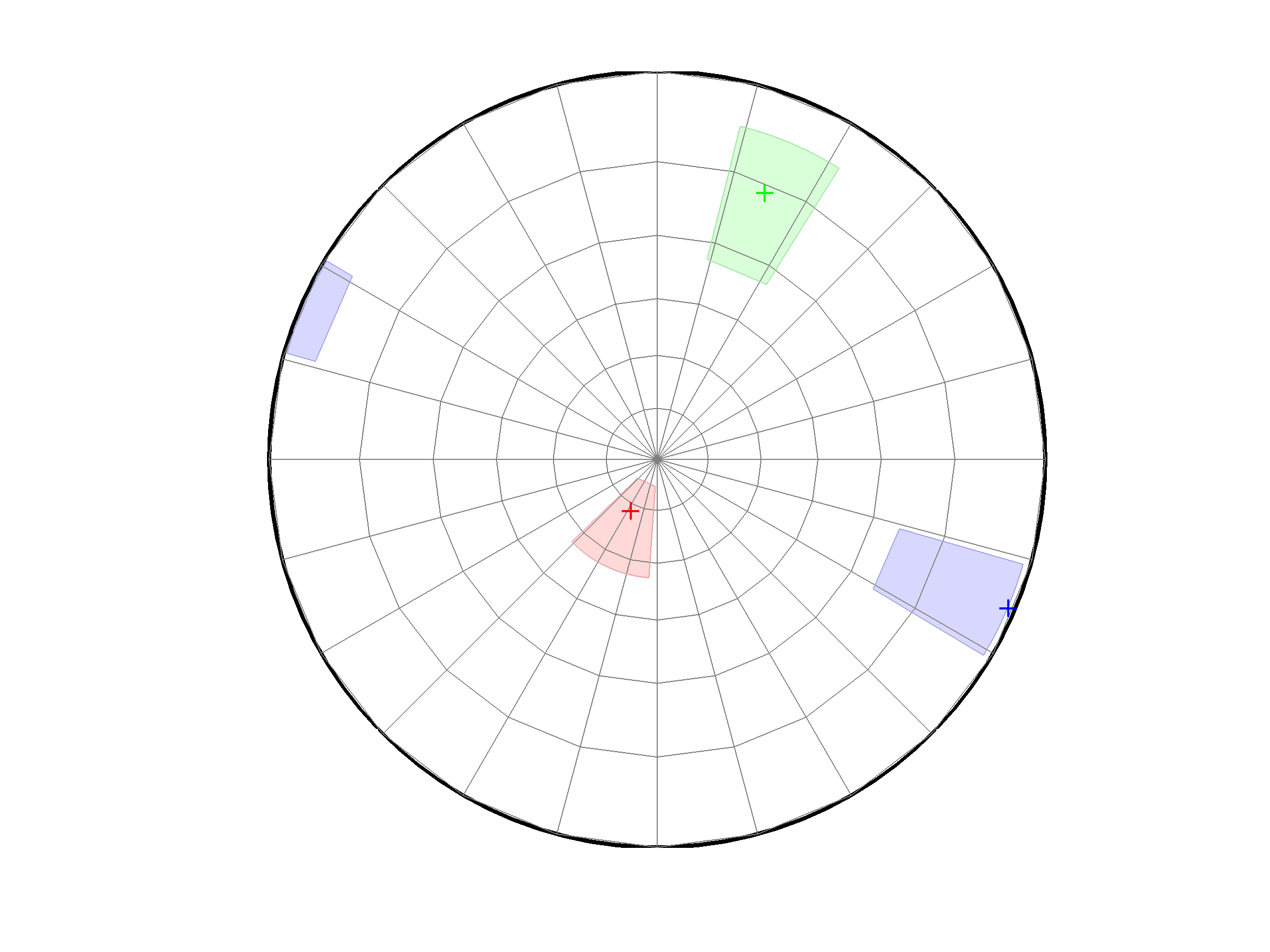
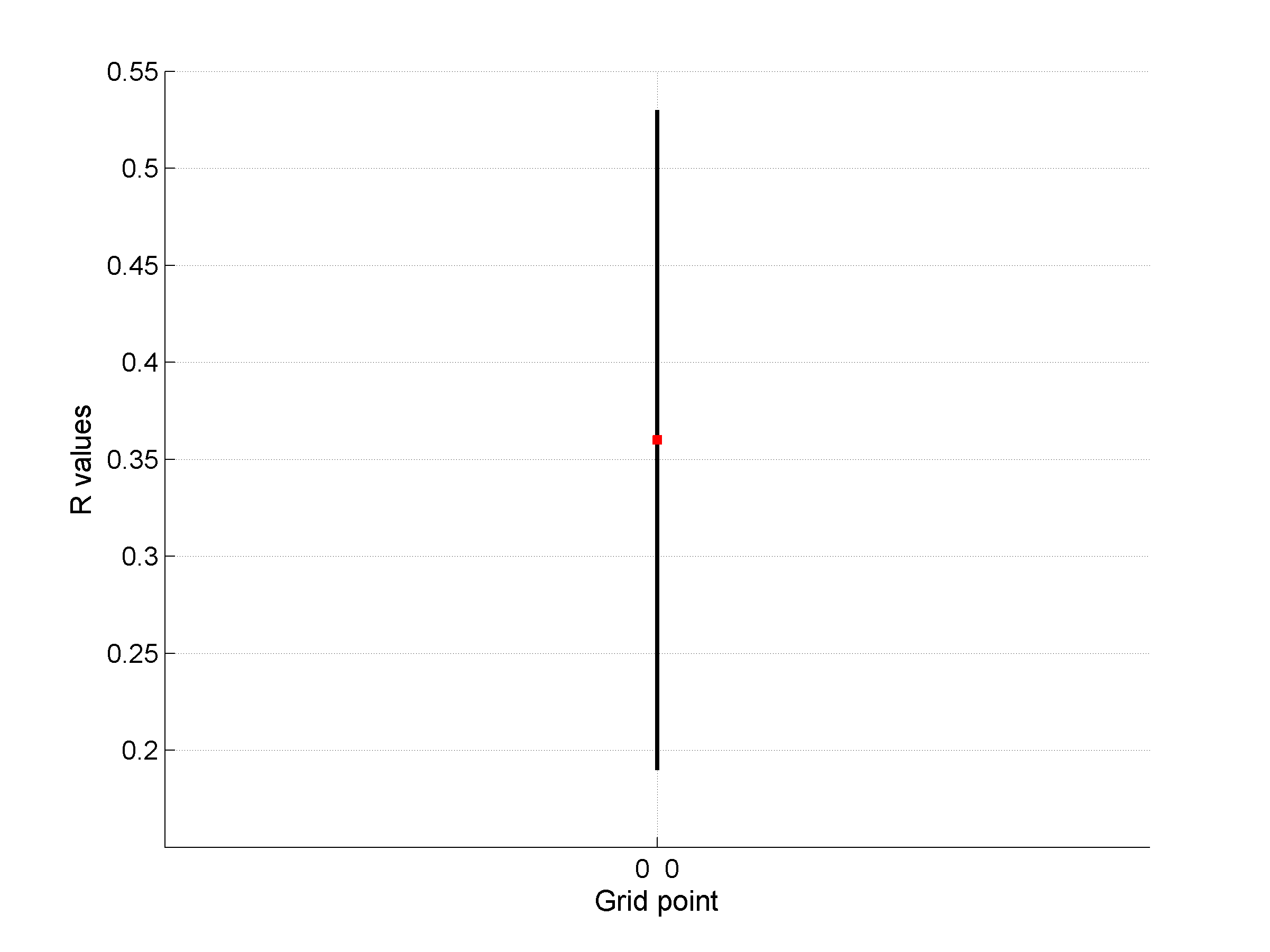
0D example of stress inversion

This example (not included in the paper) is composed of a set of 150 focal mechanisms describing normal faulting regime grouped in a single grid point [0 0]. Therefore, the problem is 0D.

To run this inversion, type:

load('INPUT_EXAMPLE0D.mat');
[OUT] = msatsi('example0',example0D,'PTPlots','on','BootstrapResamplings',2000)

Since it is only one grid point, a damped inversion cannot be performed (there are no neighboring grid points). Therefore, the ‘Damping’ is automatically settled to ‘off’ (no need to write it). As a consequence, there is no tradeoff curve output.

In this case, we have activated the P and T axis for this grid point (‘PTPlots’). The plot is contained in the folder /example0. We calculate the uncertainty by 2000 bootstrap resamplings.

Examples of plots

1 By typing:

[Hs, Hr] = msatsi_plot('example0','stereonet')

We obtain two pictures, one representing the stress and one representing R values. Examples of these are saved as ‘example0_stereonet_S.png’ and ‘example0_stereonet_R.png’

 

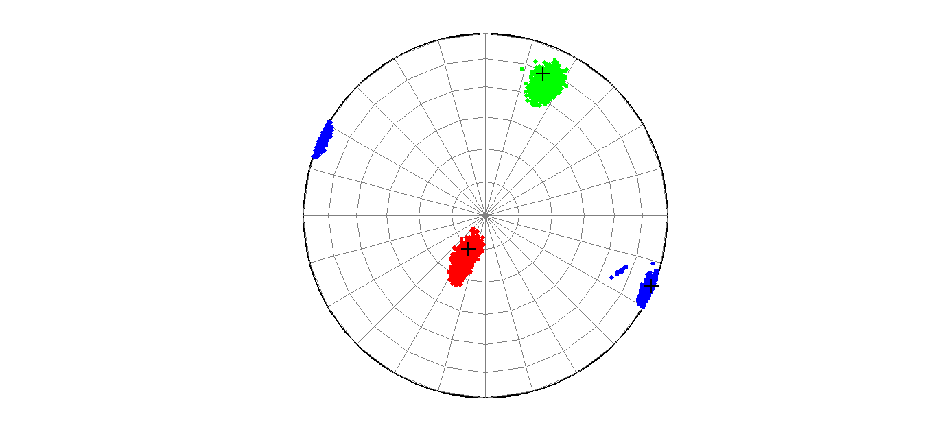
2 By typing:

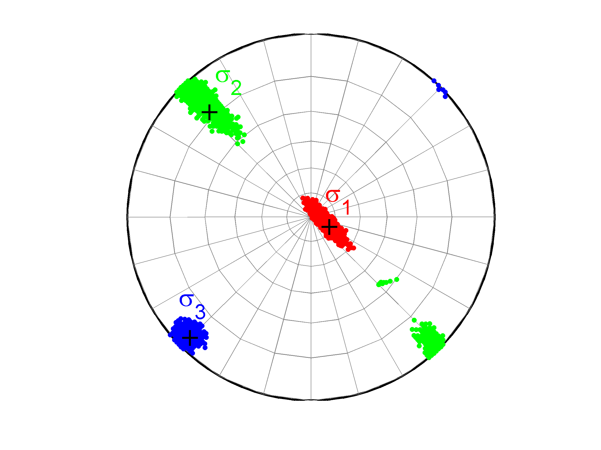
 [Hs, Hr] = msatsi_plot('example0','stereonet','ConfidenceIntervals','bootstraps')

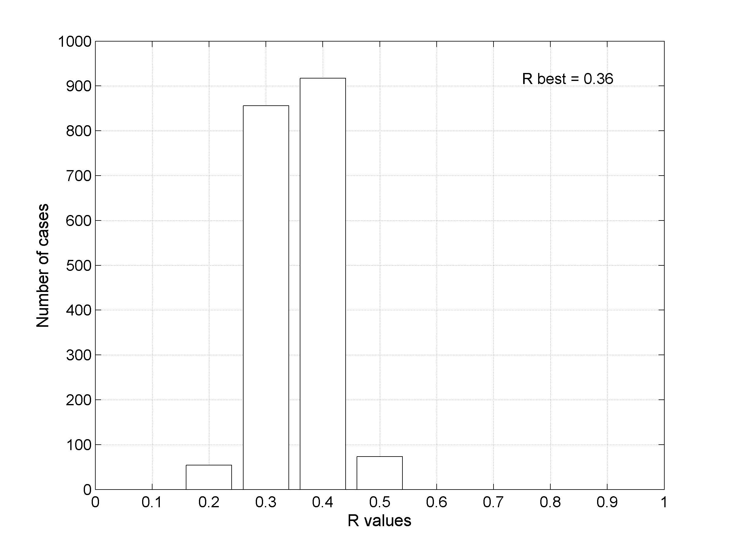
We obtain two analogous pictures as the case before but this time the uncertainties are plotted as colored dots directly from the bootstrap resampling. The R plot is a histogram. Examples of these are saved as ‘example0_stereonet_bootstraps_S.png’ and ‘example0_stereonet_bootstraps_R.png’

 

1D Example of stress inversion

This example shows the temporal stress field orientation changes at NAFZ for the co-seismic period shown in the paper. The data is part of the studies from Bohnhoff et al., (2006), and Ickrath et al., (2014).

The focal mechanisms are divided into 27 grid points that vary over the Y coordinate. Therefore, the problem is 1D. Each grid has 70 focal mechanisms.

To obtain results from the coseismic period shown in the paper, type:

load('INPUT_EXAMPLE1D.mat');

[OUT] = msatsi('example1',example1D,'BootstrapResamplings',2000)

In this case, we perform a damped inversion (settled by default) and uncertainty is calculated with 2000 bootstrap resamplings.

Examples of plots

1 By typing:

[Hs, Hr] = msatsi_plot('example1','stereonet','ConfidenceIntervals','bootstraps','SText','on')

We choose the plotting of the confidence intervals using the bootstrap resampling data. To write the name of each stress beside the data we use the property ‘SText’. We obtain two pictures for each grid point (one for stress and one for R values). Examples of these are saved as ‘example1_stereonet_bootstrap_S.png’ and ‘example1_stereonet_bootstrap_R.png’.

 

2 By typing

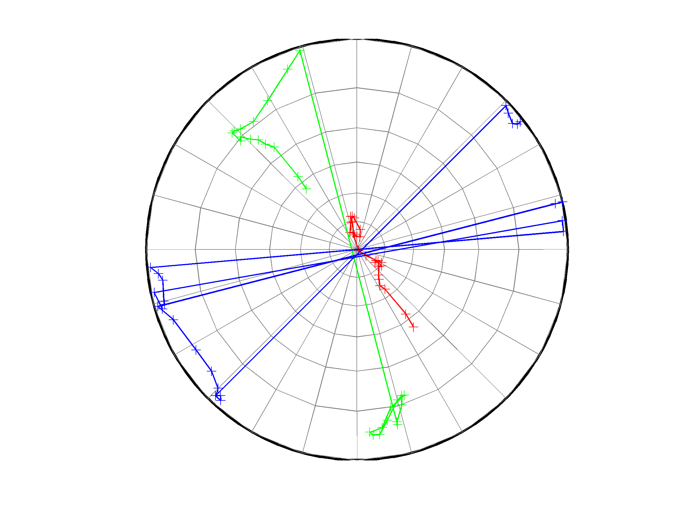
[Hs, Hr] = msatsi_plot('example1','stereonet','ConfidenceIntervals','off')

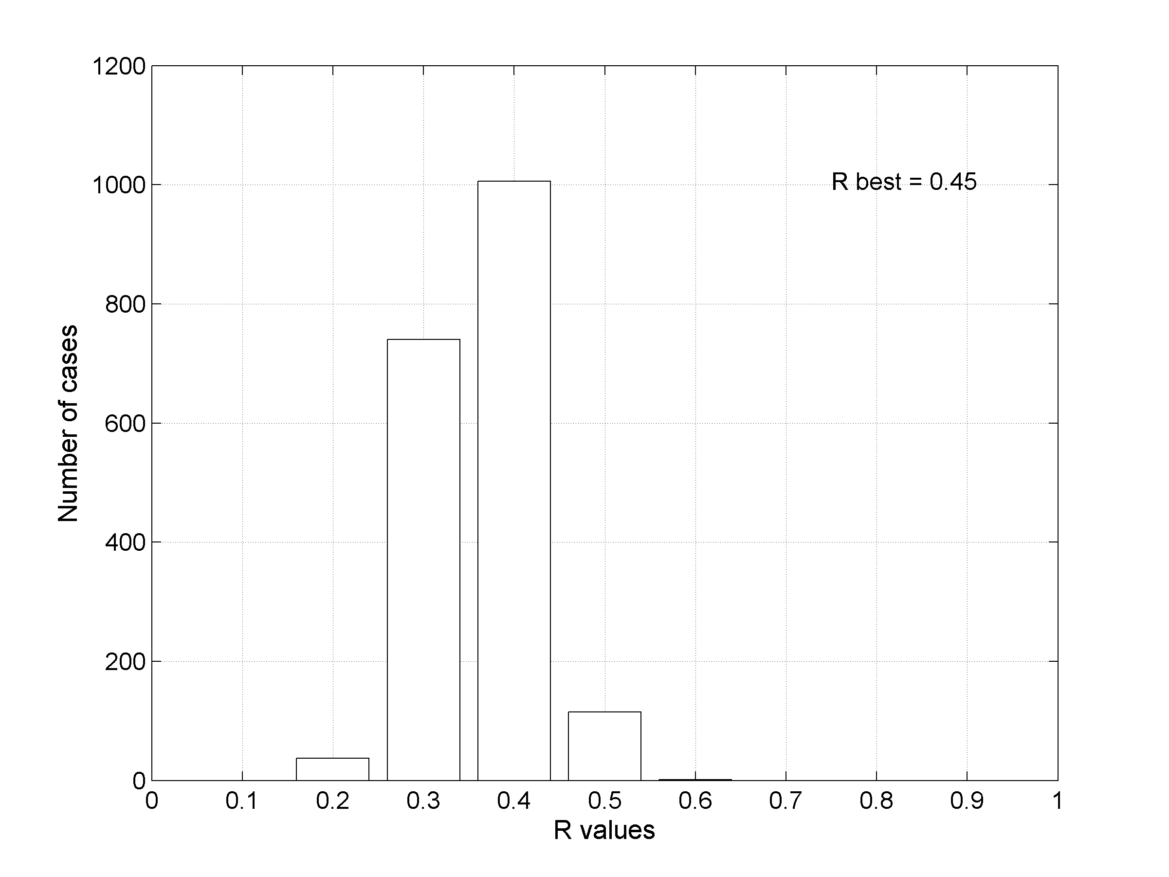
We obtain only two pictures regardless of grid point number. Since we turned off the ‘ConfidenceIntervals’, the pictures contain only the trajectory described by the best solution along the grid points. Examples of these are saved as: ‘example1_stereonet_off_S.png’ and ‘example1_stereonet_off_R.png’

 

3 By typing only

[Hs, Hr] = msatsi_plot('example1','stereonet')

We would obtain analogous pictures to those of the case before, this time together with their uncertainty intervals.

4 By typing

[Hs, Hr] = msatsi_plot('example1','profile','Title',{'This is the example n°1'})

We obtain three pictures: one for variations with trend for S1, S2 and S3 along the grid points, a second analogous picture for variations in plunge and a third one with variations in R. Uncertainties are represented with error bars.With the property ‘Title’, we have written a title we on top of each figure. Examples of these are saved as: ‘example1_profile_TR.png’, ‘example1_profile_PL.png’, ‘example1_profile_R.png’.

 

5 By typing

[Hs, Hr] = msatsi_plot('example1','profile','ConfidenceIntervals','Bootstraps')

We obtain analogous pictures as the case before, this time with the uncertainties plotted as points from the bootstrap resampling. This example was the one shown in the example from the paper.

 

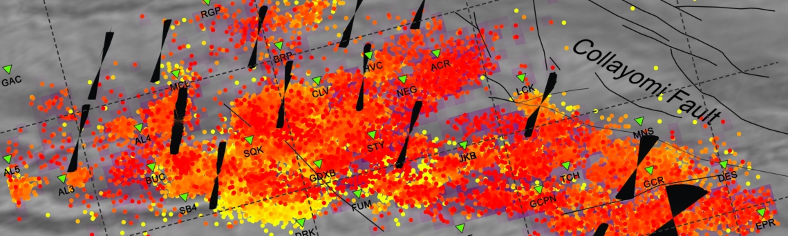
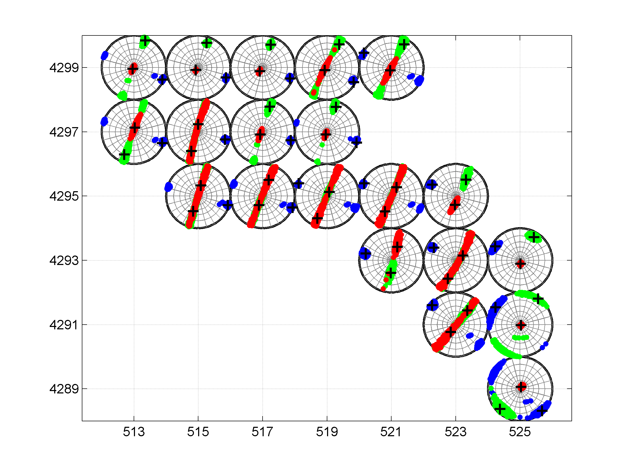
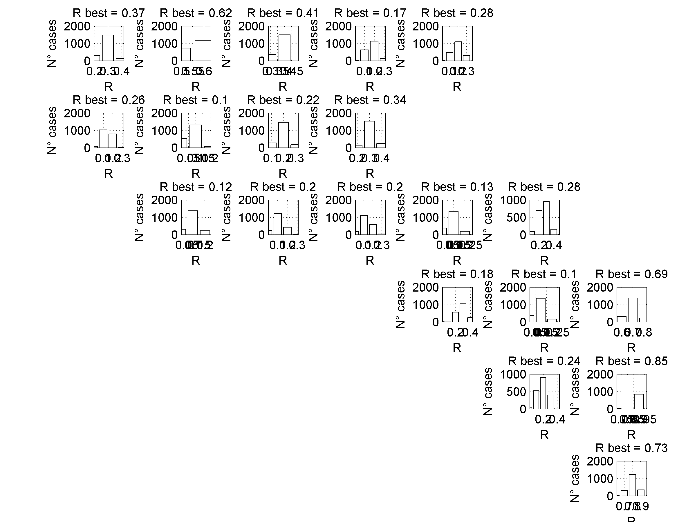
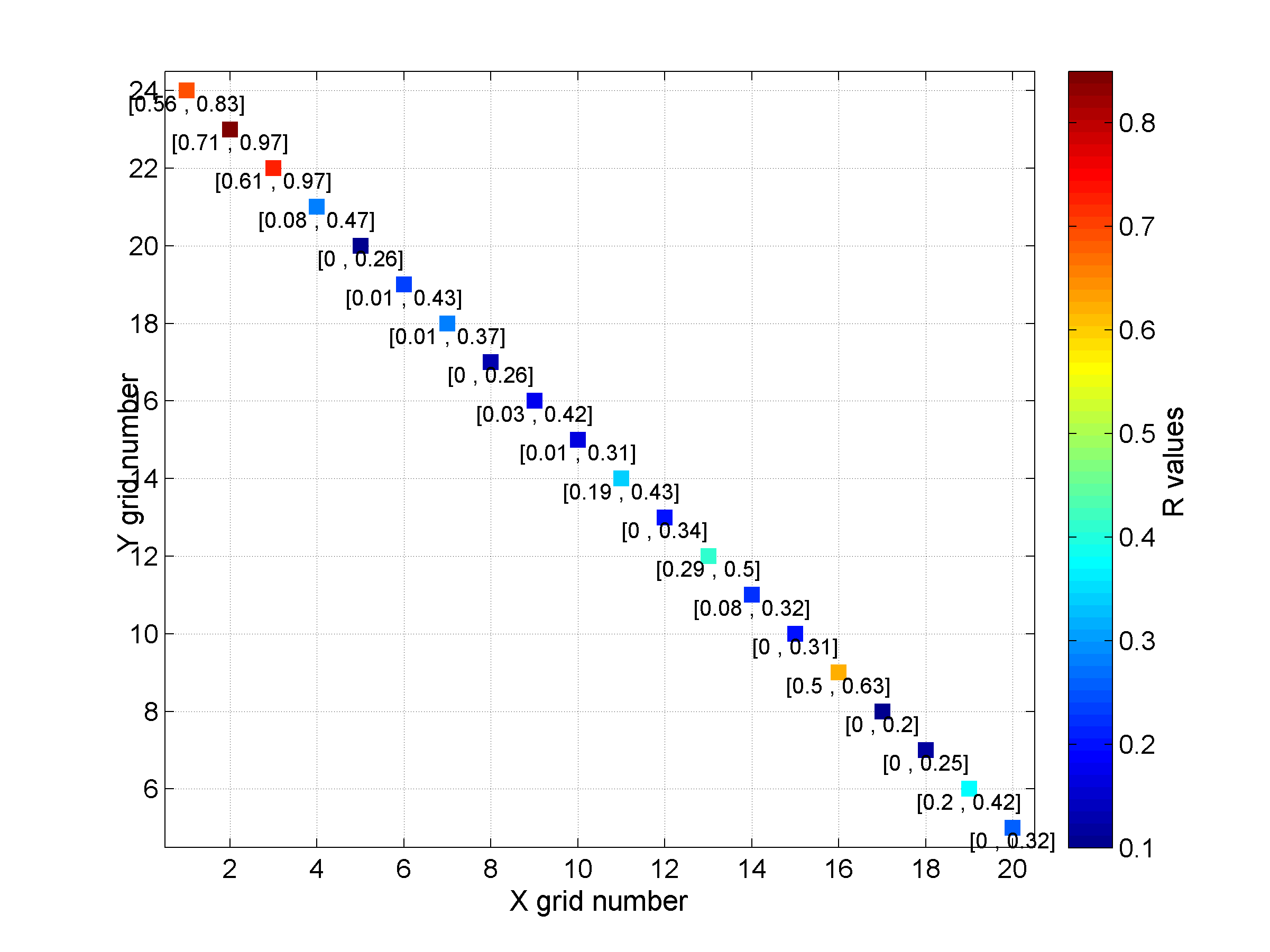
2D example of stress inversion

This example shows the surface stress field orientation at The Geysers geothermal reservoir (focal mechanisms from Northern California Earthquake Datacenter). The focal mechanisms are divided into 20 grid points that vary over the X and Y coordinate. Therefore, the problem is 2D. Each grid has a different n° of focal mechanisms (from 35 to 448).

To run the inversion of this example, type

load('INPUT_EXAMPLE2D.mat');
[OUT] = msatsi('example2',example2D,'BootstrapResamplings',2000,'MinEventsNode',30)

Here, we are also performing a damped stress inversion (by default). Uncertainty is done by 2000 bootstrap resamplings. Additionally a minimum of 30 events per node is established.

Examples of plots

1 By typing

 [Hs, Hr] = msatsi_plot('example2','stereomap')

We obtain only two pictures regardless of the number of grid points. The pictures contain one stereonet for each grid point in a map view, as well as R values. Examples of these are saved as: ‘example2_stereomap_intervals_S.png’ and ‘example2_stereomap_intervals_R.png’

 

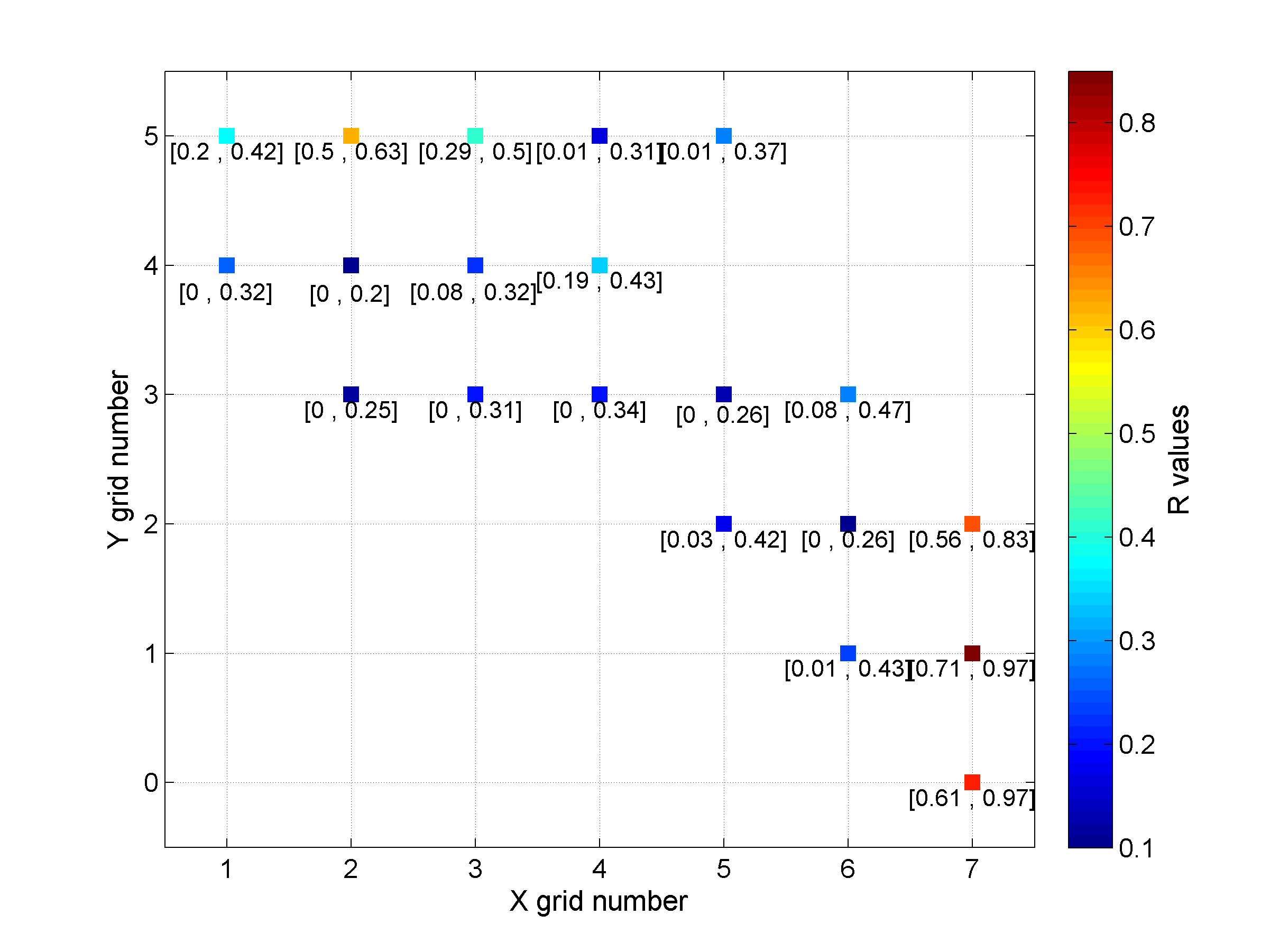
2 To create the figure from the example shown in the paper we can first define the grid label numbers (placed inside cells) and then run msatsi_plot as follows:

xgridlab = num2cell([511:2:525]);
ygridlab = num2cell([4289:2:4299]);
[Hs, Hr] = msatsi_plot('example2','stereomap','ConfidenceIntervals','Bootstraps','XgridLabel',xgridlab,'YGridLabel',ygridlab)

We obtain two pictures regardless of grid point number (one for stress and one for R values). Examples of these are saved as ‘example2_stereomap_bootstrap_S.png’ and ‘example2_stereomap_bootstrap_R.png’

 

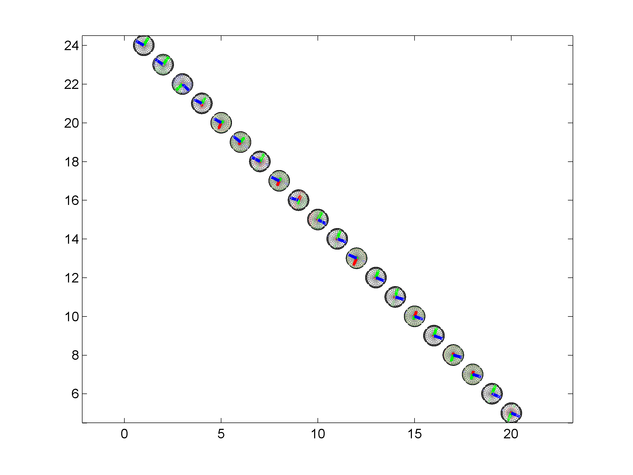
3 To place the stress inversion in any arbitrary position (e.g. their coordinates), we first create matrix with X’ Y’ (the new values to the grids ordered as OUT.GRID) and then we call msatsi_plot  as follows:

arb_grid = [(20:-1:1)',(5:1:24)'];
[Hs, Hr] = msatsi_plot('example2','stereomap','ArbitraryGrid',arb_grid,'ScaleFactor',0.5)

By playing with the value of scale factor we will achieve increase/decrease size of circles and/or overlapping of them. Examples of these pictures are saved as ‘example2_stereomap_arbitrary_grid_S.png’ and ‘example2_stereomap_arbitrary_grid_R.png’

 

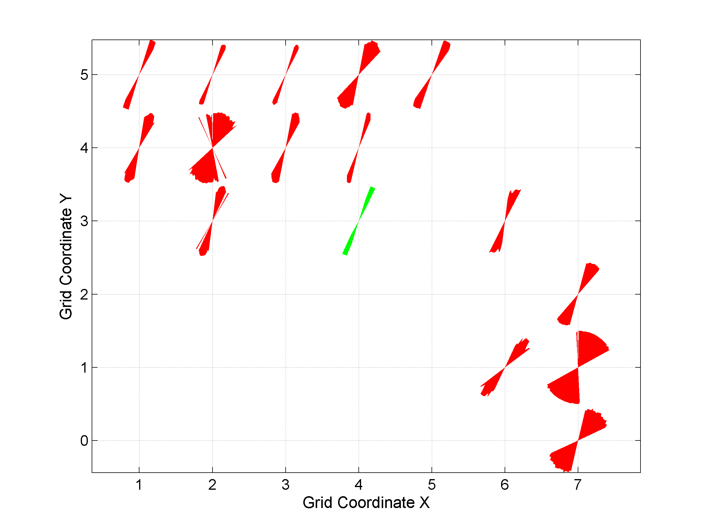
4 By typing

[Hs, Hr] = msatsi_plot('example2','wsm')

We obtain the map with the direction of maximum horizontal stresses for each grid as calculated by Lund and Townend, (2007). This example corresponds to the picture shown in Fig 6b of our paper. Example of this is saved as: ‘example2_wsm.png’

 

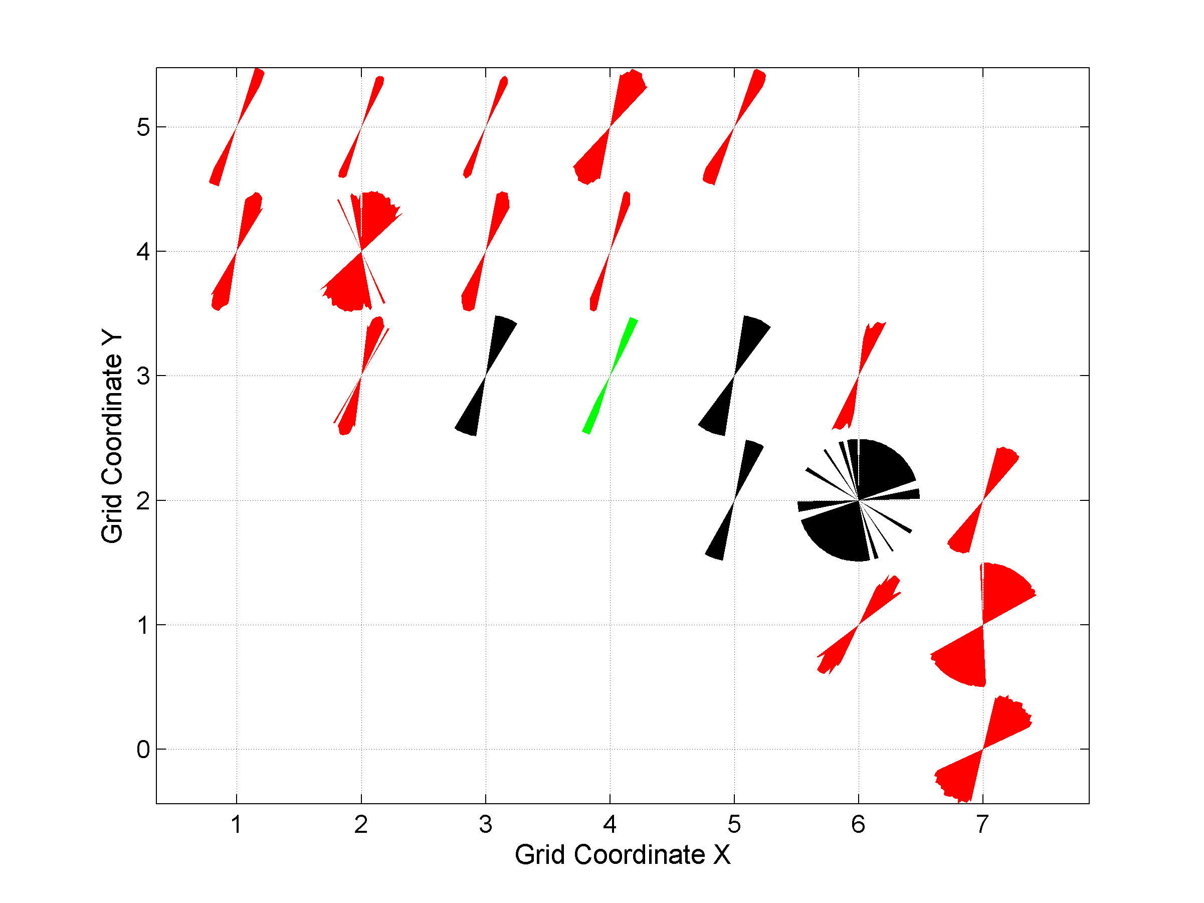
5 By typing

[Hs, Hr] = msatsi_plot('example2','wsm','IntermediateStresses','on')

We obtain the same picture as the previous example but this time also the intermediate stress inversion results plotted in black color (i.e. those not included as NF,TF or SS).

 

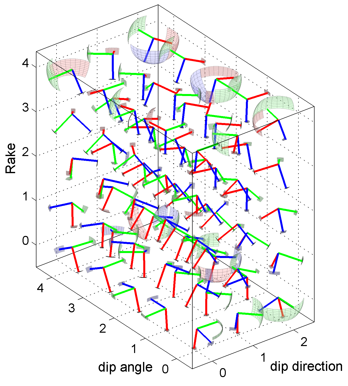
3D example of stress inversion

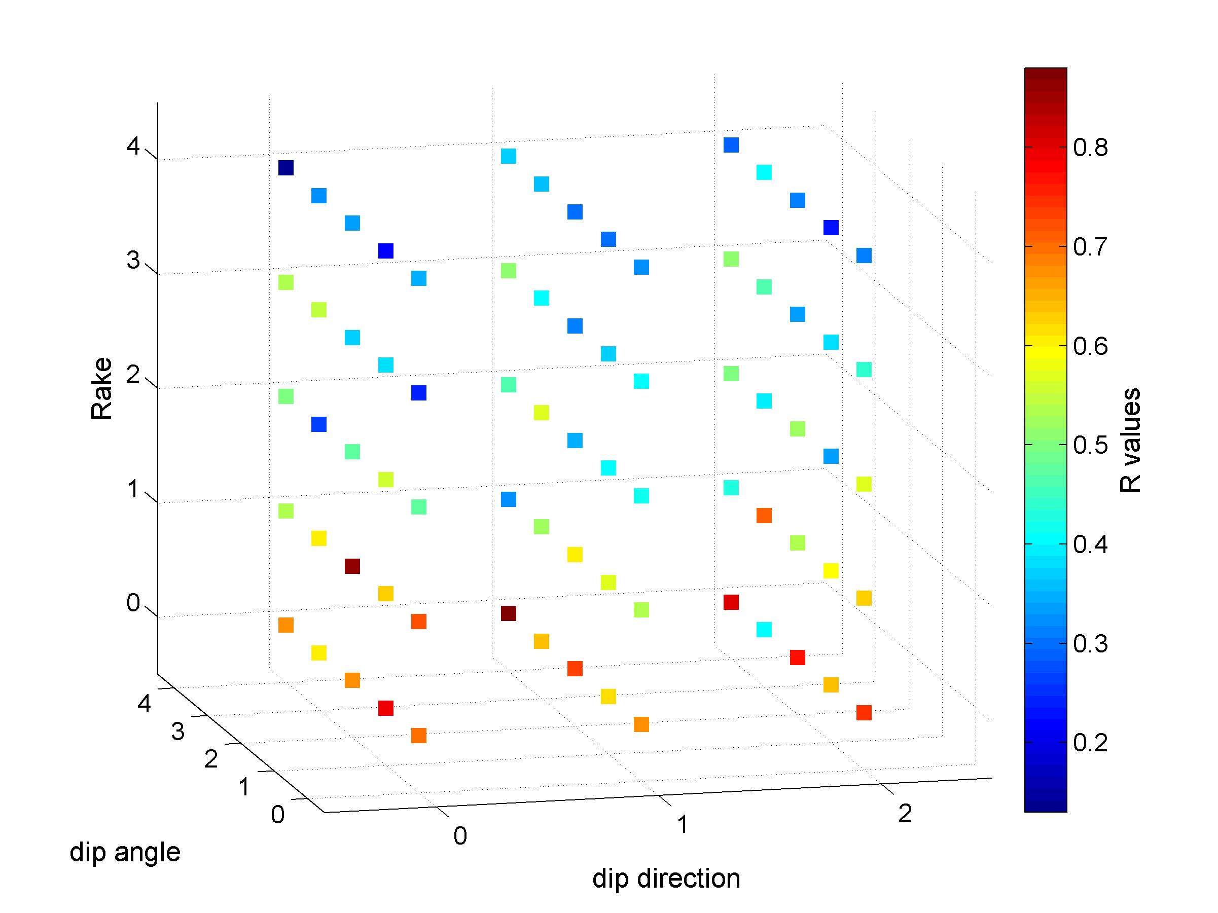
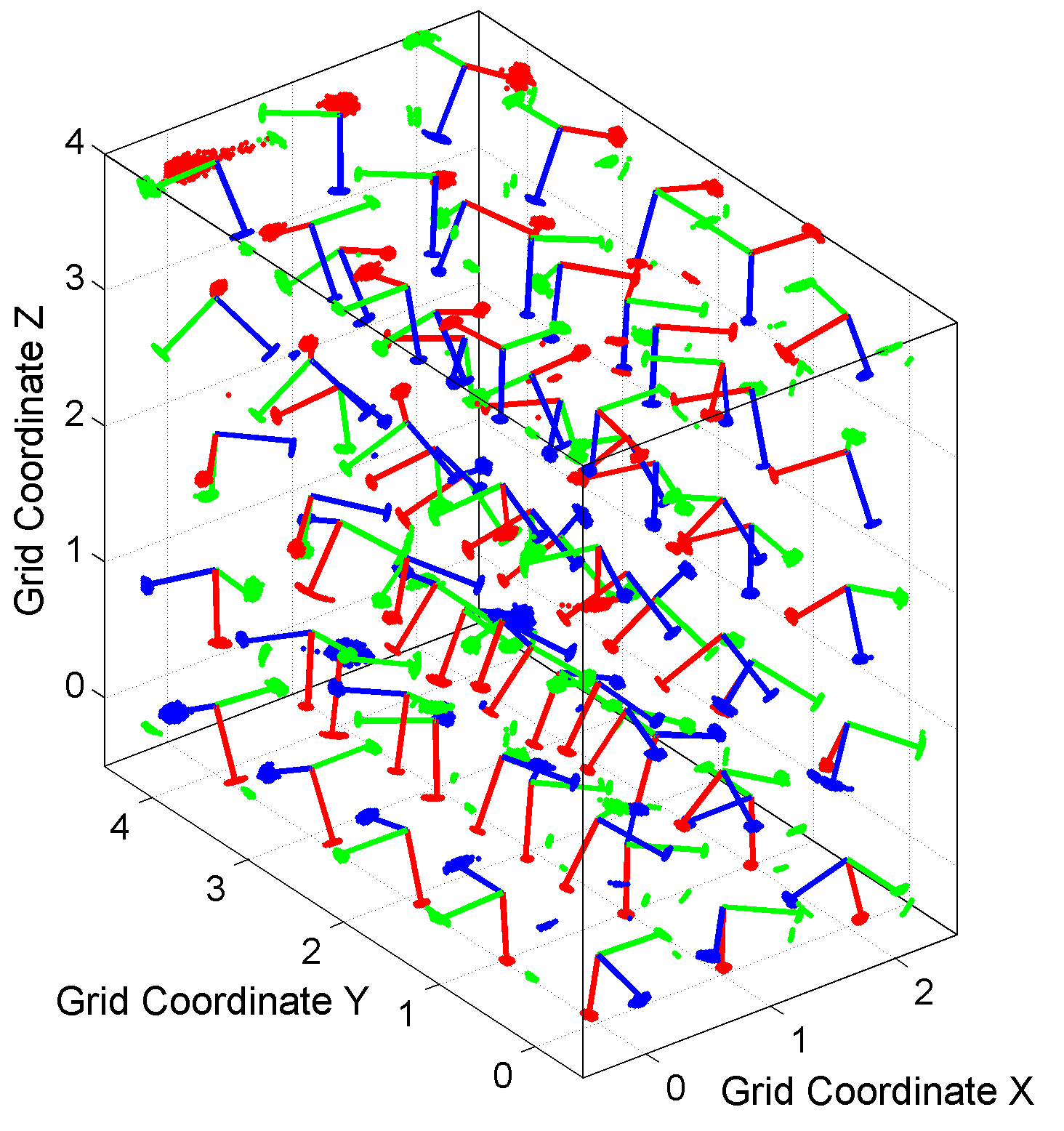
This example is a synthetic test varying the parameters of dip_direction, dip_angle and rake. The focal mechanisms are divided into 75 grid points that vary over X, Y and Z coordinates (3x5x5). Therefore, the problem is 3D. Each grid has 100 focal mechanisms.

To obtain the results shown in the paper, type:

load('INPUT_EXAMPLE3D.mat');
[OUT] = msatsi('example3',example3D,'BootstrapResamplings',2000,'Damping','off')

In this case, we have settled the ‘Damping’ off to not smooth the results of the different grids. Uncertainty assessment is performed with 2000 bootstrap resamplings.

Examples of plots

1 By typing

[Hs, Hr] = msatsi_plot('example3','stereovolume','Xlabel',{'dip direction'},'YLabel',{'dip angle'},'ZLabel',{'Rake'})

We obtain two pictures (one for stress and one for R values). We have used the properties ‘XLabel’,’YLabel’ and ‘ZLabel’ to write a label in the corresponding axes. Examples of these are saved as ‘example3_stereovolume_S.png’ and ‘example3_stereovolume_R.png’. This command was used to prepare the Fig. 7 shown in the paper.

 

2 By typing:

[Hs, Hr] = msatsi_plot('example3','stereovolume','ConfidenceIntervals','Bootstraps')

We obtain two pictures. The picture for stress shows this time the uncertainties as bootstrap resampling. R plot keeps the same as in the case before. Examples of the stress plot is saved as: ‘example3_stereovolume_bootstraps_S.png’

 

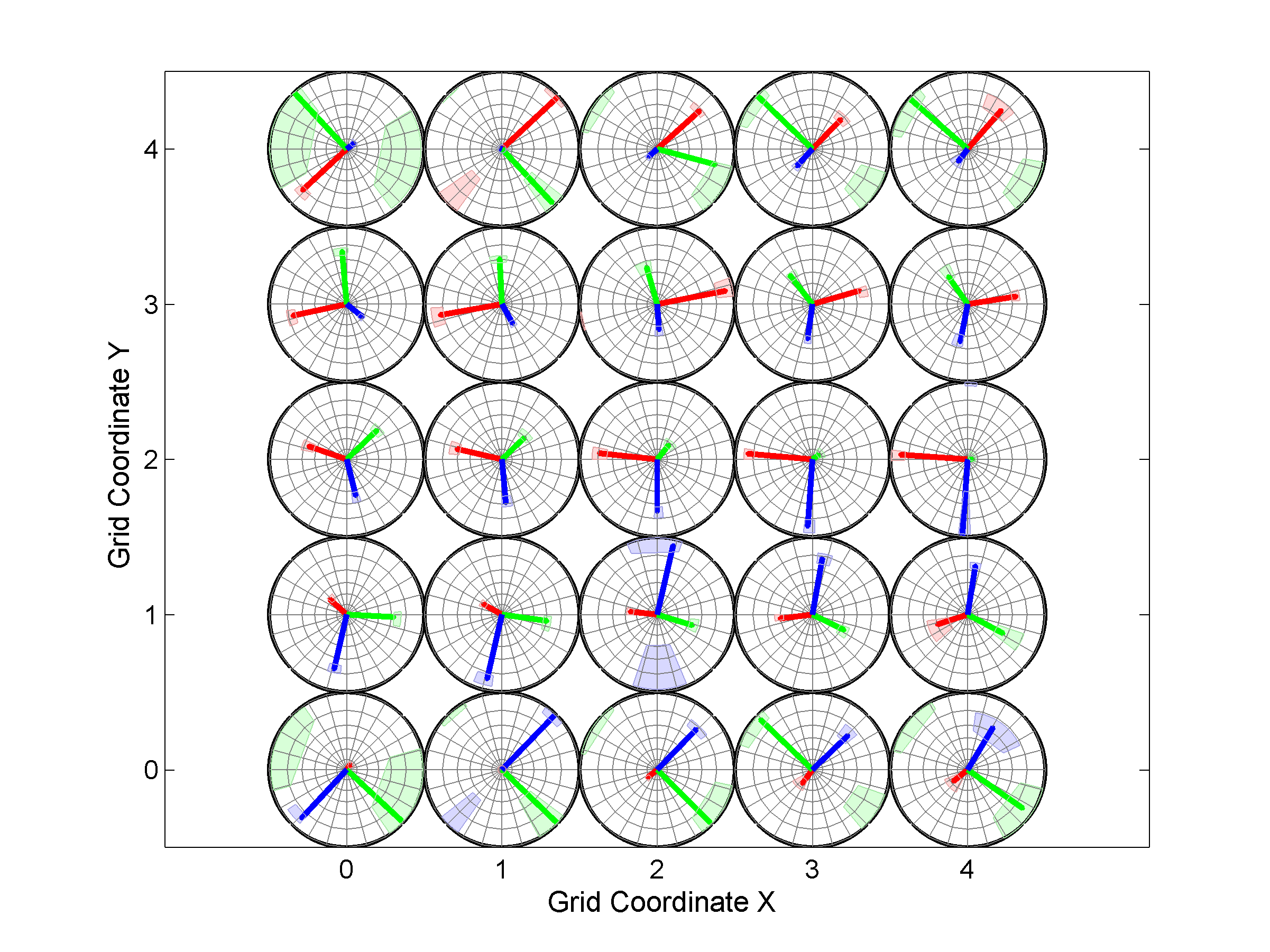
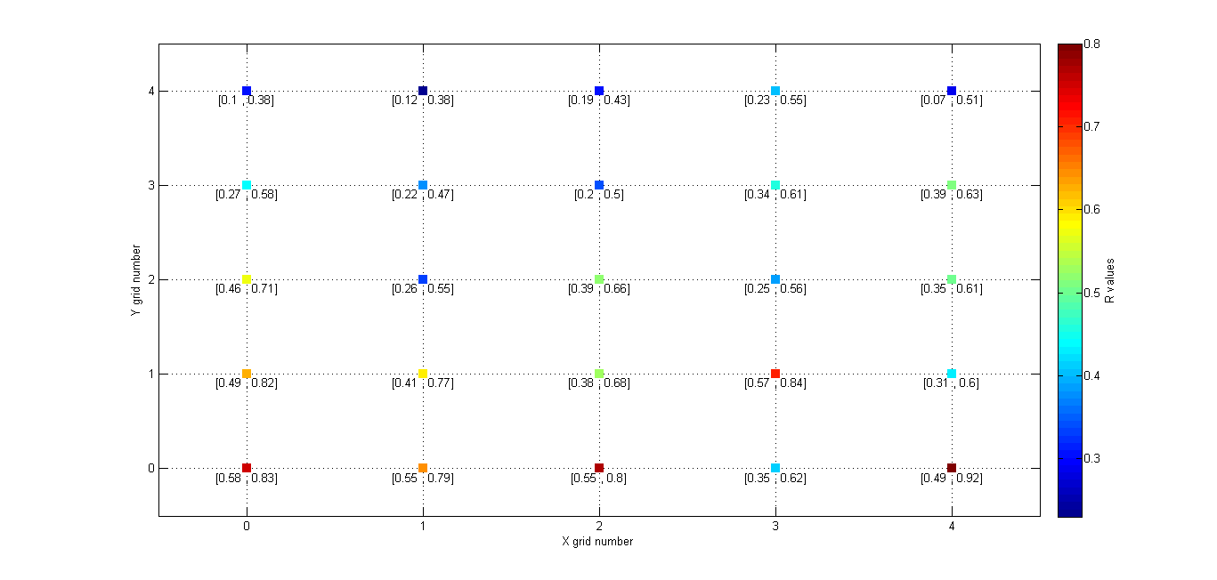
3 One useful property for 3D is ‘Slice’. In this example, we will represent only one 2D slice of our 3D results. For example, if we are interested in the inversions were dip direction = 45°, the corresponding X coordinate is 1 (because it is the second grid point). Therefore, we have to specify the condition ‘X==1’. By typing:

[Hs, Hr] = msatsi_plot('example3','stereomap','Slice','X==1')

We obtain the stereomap (2D) plot along the specified parameter. Two plots are created, one for stress and one for R values. Examples of these plots are saved as: ‘example3_stereomap_slice_X=1_S.png’ and example3_stereomap_slice_X=1_R.png

 

6. Compilation of SATSI for different platforms

The ./src directory contains modified C source code of SATSI library. Most of files have been slightly modified in comparison to the original source code developed by J. Hardebeck and A. Michael. One can download the original source files directly from the USGS website for comparison (http://earthquake.usgs.gov/research/software/). Notice that MSATSI library requires SATSI executable files compiled from MODIFIED source files (located ./src directory), therefore the original SATSI library available at USGS website and resulting executables can not be used as a replacement of the modified ones. For the convenience of the users, we provide the precompiled programs for different platforms and they are located in ./bin directory.

6.1 Compilation for Linux platform

We successfully compiled SATSI executables using GCC version 4.6.3 (Ubuntu/Linaro 4.6.3-1ubuntu5) under Ubuntu 12.04 LTS both for 64-bin and 32-bit versions. The resulting executables are available in /bin/linux directory of the MSATSI package separately for 32-bit and 64-bit version. The resulting executables should be copied to the folder containing msatsi.m and msatsi_plot.m while linux operating system is MATLAB host machine.

Compilation procedure:

1. Proceed to the ./src folder.
2. Provided that you have GCC package, execute ‘make all’ in terminal. This should create seven executable files. Warning messages may or may not appear, but they may be easily ignored.
3. Copy compiled executables to the folder containing msatsi.m and msatsi_plot.m.

6.2 Compilation for Windows platform

No procedure is provided in MSATSI package. The code was compiled following the rules from original MAKEFILE using the GCC/MINGW libraries and ECLIPSE Juno environment.

6.3 Compilation for Mac platform

1. Proceed to the ./src folder.
2. Call ‘make all’. This should create seven executable files. Warning messages may appear, but they may be easily ignored.
3. Copy compiled executables to the folder containing msatsi.m and msatsi_plot.m.

7. References

Hardebeck, J. L., and A. J. Michael (2006). Damped regional-scale stress inversions: Methodology and examples for southern California and the Coalinga aftershock sequence, J. Geophys. Res. Solid Earth 111, no. B11, B11310, doi 10.1029/2005JB004144.

Lund B. and J. Townend, (2007). Calculating horizontal stress orientations with full or partial knowledge of the tectonic stress tensor, Geophys. J. Int., 170, 1328-1335, doi: 10.1111/j.1365-246X.2007.03468.x.

Martínez-Garzón, P., G. Kwiatek, M. Ickrath and M. Bohnhoff (2013) MSATSI: A MATLAB package for stress tensor inversion combining solid classic methodology, a new simplified user-handling and a visualization tool. Seism. Res. Lett., 85, 4, doi: 10.1785/0220130189.